 Brickaizer -
Help Brickaizer -
Help |
Brickaizer -
Help
Image analysis
Image analysis
The
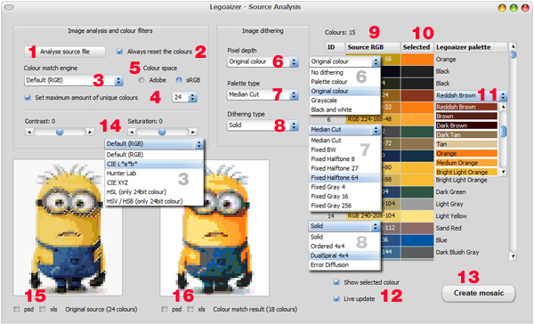
source image analysis window has a wealth of new functions. In the picture below
all these controls and settings are summarized. The source image analysis
follows a simple approach: first the source image in analysed for its colours.
Next, the colour matching is executed. The colour analysis of the picture is
shown in the image on the left, the matched colours in the image on the right.
The colours in the image are reflected in the table on the right, while the
selected matching colours from the brick palette is also shown. Mismatches are
easily spotted. Prior to showing the source image colours,
some pre-processing can be done: contrast and saturation, dithering, and colour
quantisation (or: reducing the amount of colours). Many
source images have hundreds of unique colours. When no restrictions are set on
amount of colours, the analysis can not create a colour match proposal. For that
reason the checkbox 'Set maximum amount of unique colours' is required. The
default is 24, quite a good amount for quite decent colour matches. Image
analysis
1.The
'Analyse source file'
button. By pressing this button the initial analysis is done of
the current source image. At start all the data is still empty, and
is only filled after the first analysis is completed. This button is basically a manual
analysis button, because many other parameters will automatically update the result.
2.When
an analysis is made, it takes some application parameters and settings as
input. One of these is the selected colours from the current colour palette.
This palette is the same as shown in the normal application window. When
colours are unchecked, these colours will not be taken into account for a new
analysis. By checking this box all the colours are reset. It's the same effect
as the 'Reset'
button in the normal application window. Colour matching engines
3. The
colour match engine. This is the engine to match the brick palette colours with the unique colours in the source image. The
general approach for each colour model is to compare the colour values (e.g. RGB,
HSL) with those of the brick colour palette. The colour with the least
difference is then selected as the replacement ('match') of that source image colour.
There are 6 colour engines:
4.
The checkbox to activate the maximum amount of
colours limit, and the spinbox to set the actual limit. The maximum value
is 54, as explained above.
5.
The colour space of the CIE, Hunter and XYZ colour matching engines. There are
two options: 'sRGB' or 'Adobe
RGB'
. These colour models are used in e.g. Photoshop (and
Windows) to standardize colours of images, and should be device independent. The latter
has about 40% more colours in its gamut, and will therefore provide different
colour matches (not always necessarily better!). Dithering of the source
image Image
dithering is the approach to create colour noise to avoid bands of similar
colours. In image editing applications, it's also used to elegantly reduce the
number of colours in an image.
The effect is clearly demonstrated with inkjet printers: with only 4 (or 6)
colours almost every colour can be created. The individual colour pixels are
mixed in such a way that the overall colour impression is excellent (to
the human eye). We use dithering for two purposes: to get rid of bands of
colours, and to reduce the amount of colours while maintaining the same colour impression. Although
there are three parameters to set, not all parameters can be
combined (you will notice it: nothing changes), and it's almost impossible to predict what
the effect will be for each type of image. It's a kind of
experimenting journey which dithering (and if) you prefer, and which colour matching engine will
provide that great result.
The dithering has three parameters: Colour replacement
In the table of the right you find three
columns, each serving a specific purpose. Analysis output
15.The output of the source
image analysis can be saved as a Photoshop file (.psd) where all the pixels of each colour is saved in a
layer in that file. Since the maximum amount of colours is 54, also no more than
54 layers will be created in the Photoshop file. Secondly, the same information
can also be saved in an Excel spreadsheet file (.xls), showing the blueprint numbers and
colours.
16.
Similar to 15, also the output of the matched colours can be output. This is
very similar to the spreadsheet output of the normal application
interface. Feature B. Creating a new colour brick dataset from
scratch
In some
cases you have special colours in mind and deviating bricks, which are not found
in the Bricklink database which is installed in Brickaizer. In such a case you
like to create your own dataset with colours and bricks. There is one way of
doing it, starting from a Bricklink database, and then exit, but this will very
likely fail, since the input format is very sensitive to errors. We have
now provided a very easy way to create a new dataset from scratch.
You can the new data set interface from the menu bar > 'Colour table' > 'New colour/brick
table'. This will open a very simple interface with just a
few controls (see picture above). The two
little arrows on the left indicate the size of the table. It starts by default
with 2 colours and 2 bricks (1x1 and 1x2 studs). These arrows will increase or
decrease the amount of colours and bricks. The table
in the window has 4 fixed columns: the colour name (double click and type the
colour name), the red, Green and Blue colour parameters (between 0 and 255), and
at least one the brick size. More bricks are possible, more colours as well.
There is no limit to the size of the table. Perhaps a practical size will hamper
you a bit. The values under the brick reflect the cost of each brick-colour
combination, and must be in the same value range as the one that is currently
active in your application (menu > 'Preferences'
> 'Other settings' > 'Currency x 100'). The brick sizes must be unique (errors may occur when you
have identical brick sizes), and always start with the lowest amount of studs
(so: 1x2 and not 2x1). To set a colour value a simple spin edit will show in the
cell you select. You can use the up-down arrows to quickly set the value, or
type in number between 0 and 255 (R, G, and B are provided in bytes). When you
are ready make sure all the brick values are available, and the brick names on
top of the values are correct. Only the column that has a brick value (or
rather: no text found) is taken as a table value. Then press the 'Save table as'
button and provide a name of the file. The file extension is always .xml, and
there is no need to provide it (automatically done). The table is not
automatically active, only passively saved. To change table, follow the usual
approach. Only when the table is found valid the new table will become
active.
After the source image is processed, the
colour matching starts. There are several colour matching engines, where for
some engines also the colour space can be chosen ('Adobe
RGB' or 'sRGB'
).
Finally, all the output can be saved in two distinctive
files: a photoshop file (.psd) with one colour in every layer, and the blueprint
data (.xls) which all the colours in codes, just as the normal output excel
blueprint file. There is a restriction on the amount of colours (in excel): 56.
With black and white as the reserved colours, therefore the maximum amount of
colours in the colour match is 54. The user can now change each colour by selecting a
different brick palette colour for each colour in the source image. The result is
immediately reflected in the right image.
Default RGB. Here the
Red, Green and Blue colour values are compared.
The CIE L*a*b* colour
model. This is a colour model to approximate the human colour vision. Although
it's a highly theoretical model, the practical use is that for some colours a
slightly different match is found, that somehow seems more natural.
The Hunter Lab colour
model. This is a predecessor of the CIE L*a*b* model, not necessarily worse,
but slightly different in colour selection.
CIE XYZ. One of the oldest colour models
(1931), developed to derive the colour from its wavelength. As with
the Lab models, it's also a highly theoretical approach to colour mapping,
and it can result in a very unexpected colour selection. In some cases
absolutely a great colour matching engine.
HSL or: Hue - Saturation
- Lightness. This model uses a quite different approach to defining a colour.
Rather than using the traditional red, Green and Blue it will use the Hue
('rainbow colours'), saturation and the lightness of each colour. These models
also make unexpected selections, but are useful for certain type of pictures.
The models require a colour, so these won't work with grayscale images ('8 bit
colour depth' = 256 shades of grey).
HSV or HSB. Similar
colour engine as HSL (where V = Value, B = Brightness), yet different in
colour comparison. Like the HSL model, this model only works for colour images
('24 bit colour depth' = 256 x 256 x 256 = 16.7 Mio
colours).
6.
Pixel depth. This is the characteristic of how each
pixel in the image must be treated.
The choices are 'Palette colour' (24 bit colour depth: we skip
the colour matching step by doing this directly in the dithering
step, left and right image are therefore identical. Slow but very accurate), 'Original
colour' (24 bit colour depth: a true dithering is done, using
the original source colours), 'Grayscale' (8 bit colour depth: the image is
converted into a grayscale image with 256 shades of gray, and
then dithered), and 'Black and white' (1 bit colour depth: only two
colour are used in the dithering process).
7.
Palette type. This sets the type of colour
replacement during dithering. Choices are 'Median cut' (the average or 'median'
of the surrounding pixels is selected as the representative colour), 'Fixed
BW' (only black and white pixels as output), 'Fixed halftone' (the output will
attempt to create an image with 8, 27 or 64 colours
only) and 'Fixed gray' (the output will attempt to use 4, 16
or 256 shades of gray pixels). The colour conversion for gray
dithering is unexpected, since it's looking for gray pixel matching replacements, where
the only parameter is depth of blackness.
8.
Dithering type
. This determines the shape of the dithering. Choices are 'Solid'
(practically very little colour diffusion, and bands of colour still exist),
'Ordered' (in a 4x4 pixel matrix the colour are evaluated. less banding will
occur), 'DualSpiral' (in a 4x4 matrix pixels are evaluated and clustered
together, or removed, depending of the similarity of each these pixels), and
'Error diffusion' (pixels are replaced with pixels of a different colour,
'diffusing the colours', while also the amount of colours is reduced. This
resembles the inkjet printer effect the most).
9. The source RGB. These are the original
colours (maximized to 54) of the source image. The RGB value is provided as a
reference. These are not the brick palette colours.
10. The selected matching colours of each of the
source image colours. These colours are part of the brick colour palette. In
some cases the match is perfect, while other matches are not very good. It
depends on the colour matching engine what colour is finally selected.
11. The manual colour selection. When clicking on
the third column, two things happen: all the pixels with the selected colour
is highlighted in the source image (dotted 'moving' lines), and a dropdown box
is shown. When you want to change colour with a different one, you can now
select any colour from the brick colour palette. The change is immediately
reflected in the image on the right.
12. Two additional
options are provided: show the selected colour (the 'moving dotted lines') and
'Live update' of the colour change.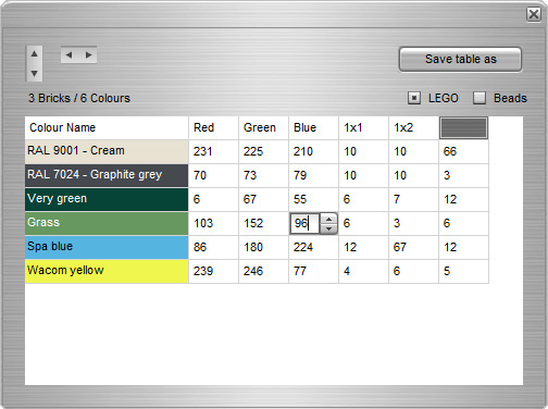
The two radio buttons indicate
what kind of table you want to create: a brick table or a Beads table. The only
difference is that in a Beads table only one type of brick is allowed: 1x1. When
you try to create a Beads table with more than one brick it will warn
you.